|
-- Original Data --
Original Data Sources - 1978
Maps and Aerial Photos
The 1978 maps showed contours at an interval of 10 meters.
The contours were labeled every 50 meters.
Due to many other line features shown on the maps, it was sometimes
difficult to determine which lines were intended as contours, especially in the
area near the Rio Grande, where contour lines were close together along
the river bluffs. The contours were
digitized using the rubber sheeted 1978 Geology map for the northern portion of
the site, and the rubber sheeted 1978 Soils map for the southern portion of the
site. (There was no geology map for
the southern portion.)
We also used some aerial photos and a mirror stereoscope to
view some of the hills and valleys in three dimensions (vertically exaggerated)
. This helped with interpreting the
contour lines. When a line on the
map was in question (concerning whether or not it was really a contour line),
the stereoscope helped to verify the landform regime and that it was or was not
a contour line (for a
small hill, arroyo, etc.)
Strategies for Field Verification
We decided to use the GPS for field verification of the contours shown on the 1978
maps. It was determined that any roads that
cross hills would be useful for
verifying the contours. For
instance, a contour line on the 1978 maps indicates the presence
of a high point (that is not really high enough to create a visible hill) along one of
the ranch roads, so we decided to drive on that road to verify the presence of
the rise in elevation indicated by the contour line on the 1978 map.
The Trimble GeoExplorer 3, used on the first field trip, has a horizontal
accuracy of one to five meters and a vertical accuracy of two to ten
meters. The Trimble XRS unit, used on the second field trip, has sub-meter
horizontal accuracy, and one- to two-meter vertical accuracy.
Strategies
for Additional Data Collection
In addition to data collected along roadways while driving, point
elevations were taken at the tops of hills using the GPS. In addition, by walking with the GPS we recorded the position and
elevation of the flowlines for the arroyos, depending on accessibility.
-- Field Work --
On the first field trip, topographical data
collection was generally guided by collection of other data. We had selected sites
for verifying soils, vegetation, wildlife and geology information, and took
these opportunities to collect topographical data at these locations as
well. Some areas were visited purely for their topographical interest, including the large hill formation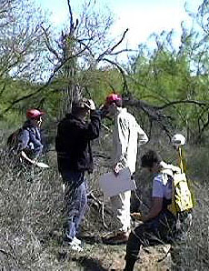 on the northern end of the ranch.
We used the GPS to record point and line features while driving
in a truck or walking cross-country, often climbing up and down hills and bluffs
to establish more accurately those areas with significant topographic
change. on the northern end of the ranch.
We used the GPS to record point and line features while driving
in a truck or walking cross-country, often climbing up and down hills and bluffs
to establish more accurately those areas with significant topographic
change.
On the second field trip a more systematic approach was used to focus on areas not previously visited. We reviewed the GPS observations from the first field trip on a laptop and chose new areas to visit and record data. We visited the hill formation on the southern end of the ranch
to make topographical observations. In addition, we verified the location of some small hills near the ranch house and recorded the flowpaths of several arroyos. We managed to get fairly good coverage with the GPS of all of the high-relief terrain, including several of the river terraces and the steeper arroyos. However, the extensive areas of gently sloping terrain are probably not adequately verified by the GPS data and we are left with only the 1978 paper maps for information in these zones.
A note on GPS data: Although we took approximately 5,000 points
of GPS data, this was not done in a uniform manner, as described above. Many of
the data points are concentrated in areas of topographical or other landscape
interest. Future field visits should take advantage of the opportunity to
expand on the GPS data by collecting additional points.
-- Data and Maps Produced --
Field Data
The field data collected was in the form of proprietary format binary files from the Trimble GPS equipment and our field notes. The field notes consisted of feature names and brief descriptions of the locations which might be useful later when trying to match up GPS data with other sampling data.
[Click here for GPS field data.]
Comparison to Existing Data
All the features collected on both the first and second field trips matched quite well with the DOQQs we obtained. It also matched up very nicely with the data digitized from the 1978 paper maps. The largest source of error identified was inconsistencies in the georeferencing process for the scanned images. The largest data offset between sources was about 4m between the GPS data and the DOQQs and about 2m between GPS data recorded on successive trips. The 2m offset was on road recordings, so it's likely that the offset there was created by the different methods used on the two trips. On the first trip, roads were recorded by holding the receiver out the window of the van, and on the second trip roads were recorded from the bed of a pickup truck.
(The first method captures data points to the right of the road, while the
second gathers information along the centerline of the road.
Data and Maps Produced
The shapefiles were in 3D-Analyst's PointZ, PolylineZ and AreaZ formats. These were used as inputs to create a TIN (Triangulated Irregular Network) description of the land surface.
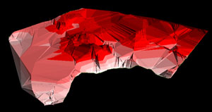 In the first attempt, all the default settings on the TIN generator were used, except that areas collected with the GPS were converted from clipping areas (boundaries for the TIN) to lines within the TIN. In the second run, all the features were broken down into the points from which they are composed and the points were used alone to generate the TIN. The differences in the results between the two methods were minute, but in a couple of places the TIN generated from points seemed to be slightly more accurate.
Relative accuracy was determined by comparison to the contour lines digitized from the 1978 maps. In the first attempt, all the default settings on the TIN generator were used, except that areas collected with the GPS were converted from clipping areas (boundaries for the TIN) to lines within the TIN. In the second run, all the features were broken down into the points from which they are composed and the points were used alone to generate the TIN. The differences in the results between the two methods were minute, but in a couple of places the TIN generated from points seemed to be slightly more accurate.
Relative accuracy was determined by comparison to the contour lines digitized from the 1978 maps.
A DEM grid (digital elevation model), contour lines, slope grid, and aspect grid were all derived from the TIN. Creation notes:
-
The cell size for all the grids was set at 10m.
-
The contour lines were generated at 2m intervals.
-
In order to create a slope grid which recorded the value in percent slope (rather than in degrees above horizontal), we copied and then modified the system script from ArcView's 3-D Analyst which generates a slope grid from a TIN.
-
The slope grid created by ArcView defaults to 9 equal-interval classes, so it had to be reclassified in order to get the detail we wanted at low slope values.
-
The aspect grid created by ArcView defaults to an 8-directional aspect class based on the cardinal compass directions. It was reclassified to reflect only
four 90-degree directional arcs: NE-NW, NW-SW, SW-SE, and SE-NE.
[Back to Top] [Home]
[Topography]
[Geology and Geomorphology] [Soils]
[Land Cover and Vegetation]
[ Roads] [Water Resources]
[Cultural Features] [Land
Uses and Practices] [Home]
|
|
-- Original Data --
Original Data Sources - 1978
Maps and 1994 Aerial Photos
The Mexican geology map covers only the northern part of the ranch, as
the map for the southern part has not yet been produced. It is scheduled to be
released by 2001. The map we had shows that three different categories of
geological features exist on the Rancho San Eduardo:

-
Lutita
(lutite)
-
Conglomerado
(conglomerate)
-
Aluvion
(alluvial sediment)
The
sandstone geologic strata that outcrop in the area are in the middle zone of a
continuum of sedimentary layers which are progressively younger as they outcrop
from the Big Bend area to the west (Paleozoic and older, more than 300 million
years) to the Gulf Coast on the east (youngest, Holocene sediments, from the
last one million years). [1], [2]
Strategies for Field Verification
Since the spatial resolution of our initial data source
was very low, the question was not to verify or to refute this information. Thus,
the development of a sophisticated field verification strategy would have
required more research than was feasible.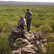
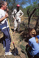
-- Field Work --
In
the field, geomorphological analysis was based primarily on observation.
In traversing the ranch, outcrops, landforms and other geological evidence was
noted visually, leading to the field description below.
-- Data and Maps Produced --
Field Data
The appearance of this geological structure in
our study area shows different layers of sandstone of tertiary age (eocene,
about 50 million years). This material is usually stratified sandstone, dipping immeasurably
to the bare eye. In some places one can find conglomerate consisting of older fluvial material
cemented in calcium carbonate. Also chert and flint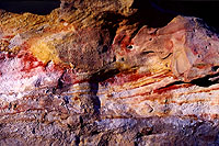 stones can be found in
various areas associated with the sandstone outcrops. The varying amount
of chalk in the sandstone as well as in the soil is possibly derived from the
high net evaporative losses in the region, leaving calcium carbonate residues in
the soil and geologic material.
The sandstone also contains a remarkable amount of
additional minerals, especially iron oxide (reddish color) and, to a much stones can be found in
various areas associated with the sandstone outcrops. The varying amount
of chalk in the sandstone as well as in the soil is possibly derived from the
high net evaporative losses in the region, leaving calcium carbonate residues in
the soil and geologic material.
The sandstone also contains a remarkable amount of
additional minerals, especially iron oxide (reddish color) and, to a much 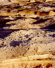 lesser extent,
manganese oxide (blackish color). lesser extent,
manganese oxide (blackish color).
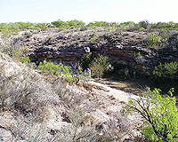
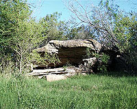
--Weathering--
This parent material has endured the forces of
weathering for many thousands of years. Due to the scarcity of water and vegetation,
water-bounded chemical weathering (hydration, hydrolysis, solution) was not the
main kind of weathering, though some stones show initial phases of a Tafoni-like
weathering (photo at right). The prevailing kind of
weathering process was and is thermal / mechanical.
--Geomorphic Evolution of the Landscape--
Material thus "prepared" could be shaped
and transported through geomorphically active forces like flowing water,
wind and gravity (in order of significance). Since the land is
quite flat in a macro-perspective, gravity probably had very little effect on the
shaping of the land. Also wind, though not to be ignored, did not
leave significant imprints on the shape of the land. The most geomorphically
active force in the study area is water, which has two main effects, erosion and
accumulation (see below.)
Erosion forms are the main characteristics in our study area,
including the erosional evolution of the Rio Grande flood channel and
floodplain. Clear signs of fluvial erosion can be seen almost all over
the area. Even on top of hills, clear signs of water erosion were found. This indicates that water from the
Rio Grande system must have reached these higher elevations in earlier times. The nearer an
observer approaches the current Rio Grande channel area, the more distinct are its effects on
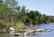
the landscape. Almost everywh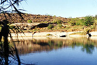 ere along its shores are more or less clearly
visible terraces that were formed in times when the Rio Grande had more water
and was prone to overbank flooding, probably during the last 50,000 years. (See
photo.) These terraces are between 10 and 100 meters wide, depending on whether they are located on the outer side of a river bend (erosional bank)
or on its inner side (accreting bank). The former is normally also more clearly
visible and mostly ends at a steep, sometimes wall-like, slope. ere along its shores are more or less clearly
visible terraces that were formed in times when the Rio Grande had more water
and was prone to overbank flooding, probably during the last 50,000 years. (See
photo.) These terraces are between 10 and 100 meters wide, depending on whether they are located on the outer side of a river bend (erosional bank)
or on its inner side (accreting bank). The former is normally also more clearly
visible and mostly ends at a steep, sometimes wall-like, slope.
|
Simplified view of the Rio Grande
|
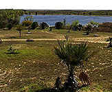
The Rio Grande valley as the deepest point in the region influences the
geomorphology in its catchment area by functioning as the local erosion base (pediplain),
that is by collecting all water from the study area. Due to the
texture of the landscape material (due to a lack of vegetation and due to the fact
that rainfall doesn't occur steadily and continuously but torrentially and very
seasonally), this water has extremely high erosional power. Several places
within
the study area showed clear signs that such events had occurred very recently,
probably in the Rio Grande flooding of October 1998. (See photo at right,
below.)
Over the years, small scars in the landscape can become deep channels that
become gorges
as fast as the landscape can move towards the pediplain.
The results are arroyos, large in number and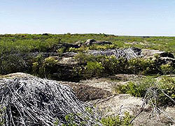 depth throughout the ranch.
The biggest ones are 10 or more meters deep over 2000 meters in length. (See
photo below, at left.) depth throughout the ranch.
The biggest ones are 10 or more meters deep over 2000 meters in length. (See
photo below, at left.)
Accumulation features could only be found
in the form of fillings in the arroyo bottoms. These fillings consist of the material
eroded from the surrounding area and from the sides of the arroyos. At
the highest points in the area (over 180 meters above sea level), conglomerate can be found, an
old accumulative phenomenon that forms a wide gravel field in its discompounded
form.
 --Anthropogenetic Geomorphism-- --Anthropogenetic Geomorphism--
Last, but not least, the anthropogenetic
interference with the shape of the landscape should be mentioned. The area of the two big irrigation fields has been leveled and planted by the Longoria family
in the 1960s, according
to unverified information. Both fields together cover more than 170 hectares. Also, many dams have been built
on the ranch as well as throughout the larger study area. Their geomorphic effect is
probably secondary because they tame the erosional power of some arroyos.
Comparison to Existing Data
A comparison to existing data is difficult if
not impossible because the information we gathered in the field is of a
different type than the maps we originally consulted. We primarily conducted
morphological observations and only in a few spots observed the actual geology.
Our findings show, however, that the map is valid as far as the geology affects
the morphology. The small hill area south of the presa is covered with a field
of gravel which can be attributed to the conglomerate shown on the map for that
location. Additionally, the alluvial sediment shown on the map close to the
river was also observed in the field.
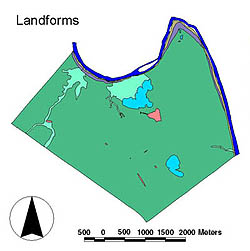
Data, Maps and Graphics Produced
In creating the geology_2000 shapefile, we did
not change the shapefile that had been digitized from the 1978 geology
map. 20 years is a geologically insignificant period of time, and we did
not observe anything in the field that made us question the map. As
mentioned above, field observations did not allow us to assess the accuracy of
the maps borders between different sedimentary rock types. The drawing
below represents our opinion about the morphology and geology of the area. In
addition, we created a shapefile named "landforms" to capture the
topographic detail of macro-geologic features, such as arroyos, hills, river
terraces and the pediplain.
Model
of a hill in the area: The top layer of rock was more resistant to
erosion, resulting in this "carved" surface.
|
|
|
References
[1] Source: H.B. Renfro: Geological Highway Map
of Texas. United States Geological Highway Map Series. Tulsa, OK, 1979
[2] Source: Bureau of Economic Geology: Geology
of Texas, Austin, 1992
[Back to Top] [Home]
[Topography]
[Geology and Geomorphology] [Soils]
[Land Cover and Vegetation]
[ Roads] [Water Resources]
[Cultural Features] [Land
Uses and Practices] [Home]
|
|
-- Original Data --
Original Data Sources - 1978
Maps and Aerial Photos
The 1978 soils maps use an international soils classification system called
FAO /UNESCO [1]. The FAO/UNESCO soil classification system was originally a soil
legend correlating the varie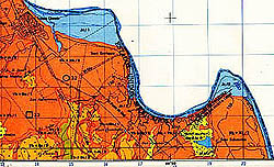 ty of soil surveys throughout the world to a common
map called Soil Map of the World. A great deal of generalization was required to
correlate the diversity of classification systems and scales of mapping to one
system. Some of the classifications do not easily translate into the
nomenclature of any particular country’s convention, nor to the U.S.
Department of Agriculture's conventions for modern county-level soil surveys. ty of soil surveys throughout the world to a common
map called Soil Map of the World. A great deal of generalization was required to
correlate the diversity of classification systems and scales of mapping to one
system. Some of the classifications do not easily translate into the
nomenclature of any particular country’s convention, nor to the U.S.
Department of Agriculture's conventions for modern county-level soil surveys.
While we based our initial observations on the UNESCO map that was published
in 1979, the UNESCO classification has since been changed. A major change has
been the removal of two first-level classes that were defined by an aridic soil
moisture regime, Y ermosols and Xerosols. This change was based on one of FAO's
general principles of their revised classification system, "that no climatic
criteria would be used to define the soil units." A majority of the study
area is composed of these two soil types. And so while the soil itself has
not changed, the use of the terms Yermosol and Xerosol is no longer accurate.
This should not prevent us, however, from characterizing the soils. ermosols and Xerosols. This change was based on one of FAO's
general principles of their revised classification system, "that no climatic
criteria would be used to define the soil units." A majority of the study
area is composed of these two soil types. And so while the soil itself has
not changed, the use of the terms Yermosol and Xerosol is no longer accurate.
This should not prevent us, however, from characterizing the soils.
Strategies for Field Verification
Given
the intricate delineations of soil boundaries on the 1979 soils maps, our strategy for field
verification was to attempt to locate areas of known soils types on the ground
and col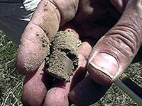 lect samples (which were then tested) to verify the types noted
on the maps. We expected to see a
wide variety of soils. However, that was not our experience. Some 25
samples were taken from locations all over the ranch (average of one sample per
200 hectares), especially where a
soil appeared unusual or near a distinct landform. lect samples (which were then tested) to verify the types noted
on the maps. We expected to see a
wide variety of soils. However, that was not our experience. Some 25
samples were taken from locations all over the ranch (average of one sample per
200 hectares), especially where a
soil appeared unusual or near a distinct landform.
Strategies for Additional Data Collection
Based
on recommendations of Dr. Stephen Hall, professor of Geography at the University
of Texas at Austin, we reviewed the Soil Survey of Webb County, Texas to
determine soil types and their qualities based on soils located immediately on
the opposite side of the Rio Grande, looking specifically in similarly
situated locations, on similarly discernable landforms.
The Webb County Soil Survey provides a wealth of data and recommendations
regarding crop productivity and native and adaptive vegetation known to grow on
those soils in that area.
-- Field Work --
 On the first field trip we drove around
the property and were able to track our location and progress accurately using aerial photographs, compass and a GPS unit.
A total of seven samples were collected using a small soil
auger to extract soil samples at depths between 5 and 20 cm. The samples
were placed in
plastic bags for later testing. Notes were taken labeling the sample and noting the
approximate location and any distinctive
features. On the first field trip we drove around
the property and were able to track our location and progress accurately using aerial photographs, compass and a GPS unit.
A total of seven samples were collected using a small soil
auger to extract soil samples at depths between 5 and 20 cm. The samples
were placed in
plastic bags for later testing. Notes were taken labeling the sample and noting the
approximate location and any distinctive
features.
A pit was dug measuring approximately 60 cm by 30 cm deep. This was done to observe the larger structure of a specific
area of soil.
On the second trip, we attempted to fill in the
gaps of missing data from what we had collected and processed on the first trip.
We used that same basic methods, however this time we also used a camera to record the appearance of samples taken. On some of the samples a field test of
calcareousness was performed using hydrochloric acid. Also we
conducted field tests of soil composition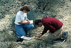 by first biting on it (if it has
a crunchy texture, then it had sand in it), then attempting to roll it to a thin
strand
about 1/2 cm in diameter (if it didn't break, the sample contained a sufficient
amount of silt) and finally squeezing it between the thumb and the index finger (if the surface was shiny, there was a sufficient amount of
clay in it). Of course, this test only provides a preliminary sense of the
texture
of the soil, but it can provide an
approximate picture of an area. Almost all of the field analyses indicated
sandy or find sandy soils, sometimes containing a small percentage of clay. by first biting on it (if it has
a crunchy texture, then it had sand in it), then attempting to roll it to a thin
strand
about 1/2 cm in diameter (if it didn't break, the sample contained a sufficient
amount of silt) and finally squeezing it between the thumb and the index finger (if the surface was shiny, there was a sufficient amount of
clay in it). Of course, this test only provides a preliminary sense of the
texture
of the soil, but it can provide an
approximate picture of an area. Almost all of the field analyses indicated
sandy or find sandy soils, sometimes containing a small percentage of clay.
One problem with the field work was the tight
timeframes we had for every stop. The soil samples had to be taken within 15 to
20 minutes which is hardly sufficient to take a sample, do the instant tests,
note everything, put it in the bag and talk with your partner about the
findings. For this reason we did not perform acid tests on calcareousness on
all of the samples. Also we were unable to take as many samples as would have
been required to produce more than a very localized view on the soil
distribution.
-- Data and Maps Produced --
Field Data
On returning from our second trip we enlisted the
services of Trinity
Engineering and Testing Company (Austin, Texas) to perform various tests on the samples. Basically, four tests were
performed:
-
The first test determined the grain size by pouring the
material through several sieves of different size meshes. The sizes were "4"
(4.7mm), "40" (0.42mm) and "200" (0.074mm). The amount left
on each sieve was measured in percentage of the whole sample. Then the material
that passed through the 200, or 0.074-mm sieve was described by
eyesight and a test on calcareousness was conducted.
-
The second test was on the Liquid Limit, which
represents the amount of water needed to make the sample behave like a liquid.
-
The third test was on the Plasticity Index. This test
determines the point at which the sample behaves like a plastic (less
water) and the point at which it is more like a liquid (more water).
-
Fourth and finally, the Atterberg Limits, which is the
Plasticity Index divided by the Liquid Limit, was determined. [Click here
for results from Trinity Engineering and Testing. (PDF Format)]
One major problem with the samples was that they were
not each individually big enough for the Atterberg test. So for this test the samples
were grouped and blended together to get at least 250 grams
each in order to perform the test. This
was done by one of the employees at Trinity by eyesight considering the grain
size and color. The samples were grouped together as follows:
-
Group 1) Sample
L, 3-b, B and J
-
Group 2) Samples
1, 3-a, 2, 4 and O
-
Group 3) Samples
D, 5
-
Group 4) Samples
6,K, A,M
-
Group 5) Samples
C1, C2, I, E
-
Only sample N had a sufficient amount for performing
the test without being blended with another.
Comparison to Existing Data
A comparison of the field data to the existing data is possible in only a very
limited way because the two data sets were prepared using different approaches. The
soil samples
taken for th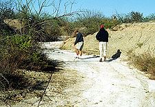 e 1978 map were taken from a much wider range of depths than 20 cm (at least
30 cm up to over one meter). Also, the 1978 tests performed on the samples were much
more elaborate as befits an official soil map. They included very detailed tests
on structure and texture, chemical processes, salinity, moisture and color,
differentiated by horizons. The
field samples alone don't provide enough detail or variability to enable
modeling of various soil-related conditions that may indicate suitability for
agricultural or settlement uses. e 1978 map were taken from a much wider range of depths than 20 cm (at least
30 cm up to over one meter). Also, the 1978 tests performed on the samples were much
more elaborate as befits an official soil map. They included very detailed tests
on structure and texture, chemical processes, salinity, moisture and color,
differentiated by horizons. The
field samples alone don't provide enough detail or variability to enable
modeling of various soil-related conditions that may indicate suitability for
agricultural or settlement uses.
Data, Maps and Graphics Produced
Although it was desirable to update the polygons on the 1978
maps, the soils team concluded that the field samples were not sufficient to
produce an updated polygon map. Instead, the samples were used to
verify/refute the 1978 mapped soil properties in regards to texture and
reactivity/ calcareousness. This was accomplished using the following
method:
Of the 80 sample points for which soils properties were analyzed
on the 1978 maps, we selected three or more sample points for each of the soil
types found on the ranch. These were selected based on proximity to the
ranch (only one of the 80 samples taken in 1978 was actually taken
within the boundaries of the ranch property) and/or contextual location--in a similar landform as the
same soil is found on the ranch. Finding that one soil sample had a surface layer texture entirely different from our
samples was considered reason enough to exclude that sample and to select another one.
Then, with three or so points for each of our soil types, we referred to the tables on the backs of the two maps
to produce a table of properties for each of the soils on the ranch. Referring to the
tables for these sample data points, we then developed a table showing the values for the
following soil properties, always referring to the upper layer of the soil (typically, the upper 0-20 cm):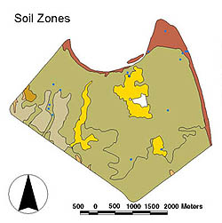
- Percent clay (arcilla)
- Percent silt (limo)
- Percent sand (arena)
- Textural classification (Ma, Mr, etc)
- Percent organic matter
- pH (acidity/alkalinity)
- Depth/thickness (profundidad)
- Reaction to hydrochloric acid (from 1 = none, to 5 = strong)
- Reaction to Calcium (in meq/100 g)
- CIC (Cation Exchange Capacity, in meq/g)
- Internal drainage properties (from very slowly drained= 0, to excessively drained = 5)
References
-
http://phylogeny.arizona.edu/OALS/IALC/soils/fao.html
-
FAO
(1974). Soil map of the world. Volumes 1-10. Food and Agriculture Organization
of the United Nations and UNESCO, Paris. 1:5,000,000.
-
FAO
(1988). Soils map of the world: revised legend. Food and Agriculture
Organization of the United Nations, Rome. 119 p.
[Back to Top] [Home]
[Topography]
[Geology and Geomorphology] [Soils]
[Land Cover and Vegetation]
[ Roads] [Water Resources]
[Cultural Features] [Land
Uses and Practices] [Home]
|
|
The original objectives of the
vegetation survey carried out in the Rancho San Eduardo were the following:
- To identify the vegetation types found in the Ranch.
- To assess the extent of each vegetation type in the Ranch.
- To produce a preliminary inventory of the plants found in the Ranch.
-- Original Data --
Original Data Sources - 1982
Maps and Aerial Photos
INEGI
Vegetation Maps (1982)
The
1982 vegetation maps, which are based on aerial photos and field observations,
provide extensive and detailed information about the vegetation cover of the
study region. The vegetation classification system used in the production of the
maps was developed by INEGI (Instituto Nacional de Estadística, Geografía, e
Informática-Mexico), and it includes categories for natural vegetation as well
as human-induced vegetation.
Thus, the maps also provide an indication of the various land uses that can be
found in the study region.
According
to the maps, between 1979 and 1982, the vegetation cover of the Rancho San
Eduardo fell into the following categories:
-
Thorn Scrublands (Either with spines or mostly thornless
)
- Matorral
Espinoso
-
Grasslands
(Either natural, induced, or cultivated) - Pastizal
-
Riparian Vegetation
- Vegetación
de galeria
-
Mesquite Scrub
- Mezquital
Almost
the entire western half of the ranch was identified as being covered by a
combination of induced grasslands and thorn scrublands (Pastizal
Inducido-Matorral Espinoso). In this same area small sectors were identified as
scrublands composed mostly of thornles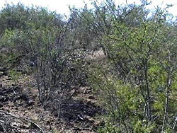 s shrubs (Matorral subinerme), and such
scrublands were sometimes identified as being found in association with induced
grasslands. Thorn scrublands were identified in scattered sectors throughout the
ranch, and were sometimes defined as being in association with either induced
grasslands or areas dominated by Opuntia
cacti (Nopaleras). Cultivated grassland (Pastizal Cultivado) was a prominent
type of vegetation identified on the ranch, particularly in the eastern half.
Only small sectors of the ranch were identified as maintaining Natural
Grasslands. A few sectors were identified as supporting an Annual Agriculture.
Some sectors were defined as Mezquitales, that is, areas where mesquite trees dominate the landscape, and portions of the
vegetation along the Rio Grande was identified as Riparian Vegetation.
Vegetation maps were digitized
using ArcView. s shrubs (Matorral subinerme), and such
scrublands were sometimes identified as being found in association with induced
grasslands. Thorn scrublands were identified in scattered sectors throughout the
ranch, and were sometimes defined as being in association with either induced
grasslands or areas dominated by Opuntia
cacti (Nopaleras). Cultivated grassland (Pastizal Cultivado) was a prominent
type of vegetation identified on the ranch, particularly in the eastern half.
Only small sectors of the ranch were identified as maintaining Natural
Grasslands. A few sectors were identified as supporting an Annual Agriculture.
Some sectors were defined as Mezquitales, that is, areas where mesquite trees dominate the landscape, and portions of the
vegetation along the Rio Grande was identified as Riparian Vegetation.
Vegetation maps were digitized
using ArcView.
All photographs were scanned for
subsequent use with ArcView files. Black and
white aerial photos from TxDOT (April 1994) were
used to identify and circumscribe sectors within the ranch that had a dense
vegetation cover. According to the
photos, the areas with the densest vegetation were found either along the river,
in association with arroyos or water tanks, or in scattered sectors in the
eastern half of the property.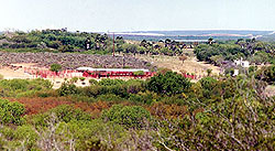
Because the team was unfamiliar
with the vegetation of the study region, the following field guides were used
to acquaint ourselves with the species native to the area. The guides include
descriptions, scientific and common names as well as color plates of the various
plants typically found in the Rio Grande Plains.
-
Richardson,
A. (1995) Plants of the Rio Grande Delta.
Austin: University of Texas Press.
-
Everett,
J. H. & D. L. Drawe (1993) Trees,
Shrubs & Cacti of South Texas. Lubbock:
Texas Tech Press.
-
Campbell
& L. Loughmiller. (1996) Texas
Wildflowers. Austin: University
of Texas Press.
Strategies for Field Verification
In order to assess the accuracy of the INEGI vegetation maps and
the information provided by the aerial photos, field verification was necessary.
To facilitate the comparison of information from both sources, a map was created
using ArcView, which incorporated the digitized vegetation maps as well as the
scanned aerial photos. The resulting map was printed for subsequent use as an
information basis during the verification process in the field.
Photocopies of the aerial photos were prepared to take into the
field. These were used to make notations about the extent of different
vegetation types found in the ranch.
Strategies
for Additional Data Collection
In order to become acquainted with the flora of the ranch, we
planned to collect voucher specimens of plants for subsequent identification and
use in the production of a floristic inventory. Therefore, a plant press and the
required collecting equipment were prepared (Refer to Methodology
& Techniques).
-- Field Work -- 
As the team surveyed the ranch by driving throughout its extent,
notations were made on the maps about the vegetation characteristics of its
sectors and the plants that appeared to dominate the landscape in each. Voucher
specimens were collected when stops were made to record GPS data or to collect
soil samples.
-- Data and Maps Produced --
Field Observations
The Rancho San Eduardo is
located in an arid region characterized by a flat terrain and a landscape of
scrublands. Although most of the area occupied by the ranch is flat, there are
sectors within it where small hills or prominent rock outcrops can be found. The
ranch is also dissected by many arroyos that open into the Rio Grande, but
which are usually dry due to the low precipitation levels in the region.
The vegetation survey revealed
that the ranch maintained different vegetation types, and that these were
usually associated with the particular geomorphic and hydrological features
of the sectors in which they were found.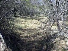 The sectors of the ranch with a level
terrain generally support open to dense scrublands dominated by mesquite and
huisache trees, while the upland sectors tend to support dense scrublands
dominated by low shrubs such as the black brush and the guajillo.
The dry arroyos maintain particular microhabitats that maintain a
distinct suite of plant species. Among these plants are hackberry and ash trees,
and many herbs that appear to prefer shaded and moist environments. This suite
of species can also be found in the areas surrounding the water tanks scattered
throughout the ranch, as well as in the sectors along the Rio Grande. In
the latter sectors, tall grasses are also a prominent feature of the landscape. The sectors of the ranch with a level
terrain generally support open to dense scrublands dominated by mesquite and
huisache trees, while the upland sectors tend to support dense scrublands
dominated by low shrubs such as the black brush and the guajillo.
The dry arroyos maintain particular microhabitats that maintain a
distinct suite of plant species. Among these plants are hackberry and ash trees,
and many herbs that appear to prefer shaded and moist environments. This suite
of species can also be found in the areas surrounding the water tanks scattered
throughout the ranch, as well as in the sectors along the Rio Grande. In
the latter sectors, tall grasses are also a prominent feature of the landscape.
Because the Rancho San Eduardo has had a long history of
being used for intensive farming and cattle raising, most of its vegetation
derives from land-use disturbances. As farming activities were abandoned about
eight years ago, large sectors of the ranch became available to pioneer species.
Differences in the time period each sector was abandoned together with
differences in previous land use, probably account for the fact that the ranch
has a landscape of scrublands in different successional stages. Areas with
pristine vegetation within the ranch are limited, and are usually confined to
sectors with an abrupt topography. The geomorphology of these sectors makes them
unsuitable for farming, and it is for this reason that their vegetation remains
undisturbed.
Vegetation Classification System
Although vegetation
classification systems generally categorize vegetation types according to their
distinct plant associations, the standards and terminology used in the
classification can vary from one system to another, depending on the purpose of
the system. In order to identify the vegetation types found on the Rancho San
Eduardo, a classification system was required. The systems that were considered
are the following:
INEGI Vegetation
Classification System
This is the standard system
currently used in Mexico for the production of fine-scale vegetation maps. The
classification is based on floristic associations. The terminology used in the
1982 maps compared to that found in INEGI’s updated system has slight
variations, but these do not appear to significantly affect the general
classification. For each vegetation category recognized by INEGI, there is a
list of plant species associated with the category. In some cases, one may find
that the species list of one vegetation type is similar to the list of another
type recognized as being distinct. However, the basis for distinguishing between
the vegetation types is the array of dominant species found in each of them.
The species lists for each of
the vegetation types recognized in the study region were obtained from INEGI’s
Geographic Synthesis of Nuevo León,
English translations of each vegetation type were obtained from INEGI’s
website.[3] [4]
Texas Parks and Wildlife
Vegetation Classification System (TPWD)
This system was developed to
produce a detailed map of the vegetation types found in Texas. The vegetation
categories recognized are based on distinct plant associations. The system
identifies various vegetation types for the Southern Plains of Texas, which are
suitable for describing the vegetation types found in the study region. A list
of plant species is associated with each vegetation type recognized in this
system, and such lists can be found at the Texas Parks and Wildlife website
Classification System
http://www.tpwd.state.tx.us/frames/admin/veg/physio2.html
http://www.tpwd.state.tx.us/frames/admin/veg/veg.html
Natural Features of the South
Plains Texas Region
http://www.tpwd.state.tx.us/expltx/sotxchart.htm
U.S. National Vegetation
Classification Standard (NVSC)
This system was developed by the
U.S. Federal Geographic Data Committee in 1997 to establish a national set of
standards for classifying the vegetation cover of the United States. The
classification is based on vegetation and floristic characteristics, not on
habitat characteristics, and it attempts to avoid land use terms. Its aim is to
provide an accurate, consistent and clear system to define the terrestrial
ecological communities of the United States. The standards of this system are
expected to be used for mapping purposes, and to be useful to those making
planning and biodiversity conservation decisions. The system is extremely
specific with regards to the definition of plant associations. Although the NVCS
is still in the process of being refined, it is already being used in various
states of the U.S. as part of an USGS-NPS mapping program. However, no national
parks in Texas are part of such program. Nevertheless, the system is being used
in Texas for various land survey purposes (Dr. Justin Williams, Zilker Botanical
Garden, pers. comm.)
Home page of the Federal
Geographic Data Committee in charge of developing the NVSC
http://www.nbs.gov/fgdc.veg/
In order to classify the
vegetation cover of the ranch according to the NVSC system, it would have been
necessary to carry-out detailed ecological studies, for which the team was
neither prepared (as we were not familiar with the flora of the ranch), nor
could we have been able to complete it successfully in the time allotted for field
work. Because the study region is located in Mexico and because discussions
regarding its development are more likely to take place in Mexico, it was
decided that the best vegetation classification system to use was the one
developed by INEGI. By using this system, the data collected in 2000 could be
compared to that presented in the 1982 maps, and would be compatible with any
vegetation maps INEGI might produce in the future. To add comparative value to
the data collected, it was decided that each vegetation type identified using
the INEGI system would be given, if possible, an equivalent vegetation type
recognized in the Texas Parks and Wildlife system.
Vegetation Types found in the Rancho San Eduardo
The following is a list of the
vegetation types identified in the ranch. Each vegetation type is identified
with the terms used by both INEGI and TPWD. A brief
description of each vegetation type as identified in the ranch is provided, as
well as information that may be useful to place the vegetation in a broader
context.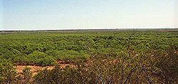
INEGI: Mezquital - Mesquite/Scrub
TPWD: Mesquite/Brush
This vegetation type dominates
the landscape of the Rancho San Eduardo. Throughout the study region, the
mesquite tree is the dominant arborescent species. It is the premier colonizer
of abandoned land, as well as the species that tends to outcompete the growth of
other plants in the region.
Large sectors of the ranch,
specially those that correspond to abandoned agricultural fields, are covered by
uniform stands of mesquite trees. The
density and height of the stands may be correlated with the time the fields were
abandoned. In other sectors, particularly those associated with arroyos and
water tanks, the mesquites tend to grow in association with other legume trees
such as the huisache, palo verde, retama, and granjeno. In the arroyo ravines,
where the environment is less arid than in the plains, the mesquite can be found
growing with elm and ash trees.
INEGI: Matorral Espinoso Tamaulipeco - Tamaulipan Thorn Scrub
TPWD: Shrub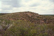
This vegetation is found mainly
in the hilly and rocky sectors of the ranch that have not been disturbed by
agricultural practices. The Tamaulipan Thorn Scrub is distributed throughout the
northern and arid regions of Tamaulipas, Nuevo Leon and Coahuila, and depending
on its composition it can be considered a climax community (Correll and
Johnston, 1979 [5] ). It is generally composed of woody plants less than three
meters tall,
the majority of which are armed with thorns. Among the prominent species
identified in this vegetation type are the chaparro prieto, granjeno, amargoso,
guayacan, retama, cenizo, coyotillo, guajillo, nopal, vara dulce, huizache,
gobernadora, jatropha.
INEGI: Vegetación de Galeria - Riparian Vegetation (Natural)
TPWD: Marsh (Possibly Swamp according to their broad definition)
 This vegetation is found along
the Rio Grande and it is quite distinct from that found in any other
sectors of the Ranch. Among the plants commonly found in this community are tall
grass species (Airside?), Parkinsonia
and mesquite trees, Acacia shrubs, and
a variety of herbs including the tobacco tree. This vegetation is found along
the Rio Grande and it is quite distinct from that found in any other
sectors of the Ranch. Among the plants commonly found in this community are tall
grass species (Airside?), Parkinsonia
and mesquite trees, Acacia shrubs, and
a variety of herbs including the tobacco tree.
According to the U.S. Fish and
Wildlife Service, riparian areas are “plant communities contiguous to and
affected by surface and subsurface hydrologic features of perennial or
intermittent lotic and lentic water bodies (rivers, streams, lakes, or drainage
ways). Riparian areas have one or both of the following characteristics: 1)
distinctively different vegetative species than adjacent areas, and 2) species
similar to adjacent areas but exhibiting more vigorous or robust growth forms.
Riparian areas are usually transitional between wetland and uplan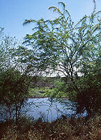 d." d."
INEGI: Vegetación de Galeria - Riparian Vegetation (Induced)
TPWD: Marsh
This vegetation type is distinguished from the Natural Riparian Areas only because they are found in
association with human-made water tanks. This distinction is not made by INEGI.
INEGI: Pastizal Natural - Natural Grassland
 TPWD: Grassland TPWD: Grassland
The matrix of the vegetation
found throughout the ranch is that of short grasslands. The actual species
composition of these grasslands is not clear, as not many voucher specimens were
collected in it. However, it is likely that Hilaria, Bouteloua, Aristida and
Buchloe will be among the grasses
found in this vegetation type.
INEGI: Pastizal Inducido - Induced Grassland
TPWD: Grassland/Other Native or Introduced Grasslands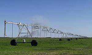
This vegetation is maintained
either to provide a source of food for the herd of cattle in the ranch, or as a
landscape feature in the areas surrounding the house and work structures of the
ranch.
INEGI: Nopalera - Prickly pear cacti area
TPWD: None
This category of vegetation is
not included in the broad vegetation classification of INEGI, but is used in the
1982 maps. It is a useful term to use in conjunction with other vegetation
categories to reflect that the area has a significant component of Opuntia
cacti, or to describe areas that are planted with these cacti.
Other Vegetation Cover
 A type of vegetation that is not
recognized by the INEGI system, but which might be useful for describing some
sectors in the ranch is that of Induced Vegetation. This term can be
particularly useful for referring to the sectors where non-native plants are
cultivated for aesthetic purposes, such as the areas closest to the main house
and main water tank, including a pecan orchard. A type of vegetation that is not
recognized by the INEGI system, but which might be useful for describing some
sectors in the ranch is that of Induced Vegetation. This term can be
particularly useful for referring to the sectors where non-native plants are
cultivated for aesthetic purposes, such as the areas closest to the main house
and main water tank, including a pecan orchard.
Floristic Inventory
During the two visits to the
Rancho San Eduardo, a total of 45 voucher specimens were collected. Specimens
were identified using Correll and Johnston’s Manual of the Vascular Plants of Texas, and were compared to
specimens in the Herbarium of the University of Texas to verify their identity.
The resulting floristic list includes 34 species [Click
here to view the floristic inventory].
GIS Maps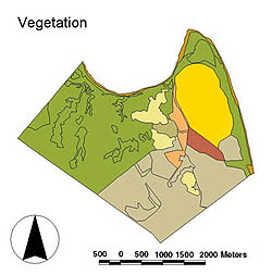
An updated vegetation map of the
Rancho San Eduardo was produced using ArcView. The data used to produce the map
include the notations made during the visits to the ranch and vegetation density
information obtained from 1997 digital orthophoto quads and infra-red photos
produced by INEGI in 1998. The last two sources were not used until the final
phase of the project. In the new vegetation map, polygons represent distinct
vegetation types as were observed in the field. The delineation of the polygons
must not be considered to be precise, as their extent was not defined by GPS
data. Different plant densities which could be recognized in the infra-red
photos were also defined as distinct polygons, and were identified as
maintaining a high, low, or medium density. An effort was made to distinguish
areas with natural vegetation from areas with induced vegetation.
Verification/Inconsistencies
Because the original vegetation
maps were produced almost twenty years ago, and in the period that has lapsed
the ranch has undergone many land-use changes, it was expected that the
vegetation cover would not be the same as that depicted in the 1982 maps. It is
difficult to ascertain if the 1982 maps had any inconsistencies, given that
vegetation cover can change dramatically in twenty years. However, it was found
that the vegetation types identified in the 1982 maps were still present in the
ranch, with the exception of the cultivated areas.
The sectors identified in 1982
as being covered by a combination of induced grasslands and thorn scrublands was
found to be much reduced today. This can be attributed to the fact that farming
practices in the ranch have been abandoned, and that previous agricultural
fields have been taken over by mesquite trees. The eastern half of the ranch
which was identified as maintaining cultivated grasslands is today mostly
devoted to the maintenance of grass for the cattle on the ranch. Thorn
scrublands were identified throughout the ranch in 1982, and these are still
present although their specific delimitation requires further field work.
[3] Main Vegetation Types (INEGI)
http://ags.inegi.gob.mx/sinegi/territorio/ingles/fiterritorio.html
[4] Sintesis Geografica de Nuevo León (1981) Mexico City: Secretaría
de Programación y Presupuesto; Coordinación General de los Servicios
Nacionales de Estadistica, Geografía e Informatica. (A hard copy is available at the
Plant Resources Center of UT. Contact the Curator.)
[5] Correll, D.S. and M.C.
Johnston. (1979) Manual of the Vascular Plants of Texas. Richardson: The University
of Texas at Dallas.
[Back to Top] [Home]
[Topography]
[Geology and Geomorphology] [Soils]
[Land Cover and Vegetation]
[ Roads] [Water Resources]
[Cultural Features] [Land
Uses and Practices] [Home]
|
|
-- Original Data --
Natural Water Features
Rio Grande
A digital geographic file delineating the Rio Grande was originally
obtained by scanning the 1978 Mexican thematic maps and then digitizing the
shoreline of the river as shown on those maps. The originally digitized
shapefile from the 1978 maps was up to 40 meters off in many lo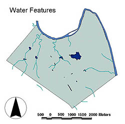 cations, so the RioGrande_2000 shapefile was
revised by
adjusting the northern RioGrande_1978 shapefile to match the water surface
boundary shown on the San Pedro Hill DOQQs.
The originally digitized shapefile from the 1978 maps was up to 40 meters
off in many locations. If the
remaining DOQQs become available for the site, the southern portion will need to
be adjusted similarly. The easiest
way to adjust the boundary is to make the river polygon clear and increase the
outline width to 3. With the blue
color of the water surface showing through beneath the polygon, the outline can
be adjusted to match the edge of the water surface on the DOQQ. cations, so the RioGrande_2000 shapefile was
revised by
adjusting the northern RioGrande_1978 shapefile to match the water surface
boundary shown on the San Pedro Hill DOQQs.
The originally digitized shapefile from the 1978 maps was up to 40 meters
off in many locations. If the
remaining DOQQs become available for the site, the southern portion will need to
be adjusted similarly. The easiest
way to adjust the boundary is to make the river polygon clear and increase the
outline width to 3. With the blue
color of the water surface showing through beneath the polygon, the outline can
be adjusted to match the edge of the water surface on the DOQQ.
Arroyos
As
discussed in the geology and geomorphology
section, the ranch has several natural arroyos which are still enlarging as a
result of erosive floodwaters. In many localized places, ranch workers have
attempted to control erosion, with some success.
Much more remediation is still possible and would be very beneficial
 Livestock
Tanks Livestock
Tanks
The
livestock tanks were originally digitized using the 1978 maps.
Based on the 1994 and 1997 aerial photos, the livestock tanks were re-digitized to create
the tanks_2000 shapefile. Five of
the tanks shown on the aerial photos were not shown on the 1978 maps (ID = 7-11
in shapefile). One other tank was
shown on both sources (ID=14 in shapefile), but it was about 170 meters
displaced. This may have been an
error on the 1978 maps, or perhaps the tank was relocated since 1978.
Floodplains
Floodplain data was not available from
the IBWC, so we searched for a map at the FEMA website (www.fema.gov), locating
a map for the U.S. side of the Rio Grande at the project location.
We also obtained a copy of the FEMA floodplain map from the TNRIS center
for the U.S. side of the Rio Grande. The FEMA map showed the approximate
location of the 100-year floodplain, which we scanned and rubbersheeted to match
our other maps. Unfortunately, the
map appeared to be very crude and did not rubbersheet very well. Elevation data was not available on the FEMA map, so we
obtained the USGS map for this area and rubbersheeted it as well.
The USGS map was of much higher quality and rubbersheeted quite nicely.
We estimated the floodplain for our site by roughly measuring the
distance from the edge of the floodplain from the river on the FEMA map, and
then approximating the elevation by looking at the elevation on the USGS map.
Once we had estimated the floodplain elevation in feet (U.S. info), we
converted it to meters and then drew the approximate floodplain on the Mexico
side using the contour file that was derived from the 1978 maps.
Note: The 1978 contours are
also shown on the USGS map, which states "Mexico portion copied from DGG
1:50,000 scale map, Villa hidalgo G14A17, dated 1978."
For the arroyos on the site, we did not
have cross sections of the arroyos, so we could not calculate the floodplains
for them. We have not yet obtained
historical rainfall data for the site either.
In order to have something to plug into the suitability models, we
selected a buffer of 40 meters for the arroyos as an approximate floodplain.
The location of the arroyos were sometimes difficult to determine from
the DOQQs, so part of the reason for having such a large buffer was that the
centerline of the arroyo might be far away from the lines we drew on the
“waterlines” file. The actual
floodplain will be determined by future work for the site, once further data has
been collected.
Waterworks System
The 1978 maps were not detailed enough to include in
formation
about the waterworks. Such data was therefore not
digitized like many of the other themes. Instead, data was collected during the two field trips.
-- Field Work --
Field work consisted of noting the locations of pumps, wells, a
pumphouse, livestock watering tanks, etc. This information was primarily recorded using the GPS device, while notes were
also recorded on maps. Personal interviews with the ranch manager provided additional technical information (pipe diameter, location and control switches) about operating and non-operating acequias
(irrigation ditches) and the irrigation system currently in use.
-- Data and Maps Produced --
Field Data
The following report was composed from an interview with the ranch manager
concerning the waterworks on the ranch, recorded during a driving tour of the ranch facilities.
At the pump house on the bank of the Rio Grande, there are
two electric pumps (from 1982) and one older diesel pump. Only the electric ones
are in use nowadays. These two pumps are used in alternation to keep them in
working order, but are not used simultaneously because the water produced would
overflow the storage tank. The water intake structure is located below the pump
house, at and below the river level. Each electric pump has a capacity of 3,000 gallons per
minute. The water is pumped into a preliminary holding tank or standpipe housed in a white
building on the east side of the road next to the pump house.
Preliminary storage is at roughly the same elevation as the irrigation
fields. From this structure, there are two main paths for the water.
1) One path leads to the center pivot irrigation fields. There are two
fields, one larger than the other. From the preliminary tank, a 15.5-inch
diameter underground pipe runs to the center pivot of the northern irrigation
apparatus. From there, a 10-inch diameter underground pipe runs to the center of
the southern irrigation field.
2) The other arm of the water system begins with a 24-inch
pipe coming from the preliminary storage tank and travels south along the
perimeter of the irrigated area until it comes to a manhole (location marked
pump 2 on the map). There is normal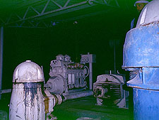 ly a pump at this location, but it is under repair now. From pump 2, the water
runs through a concrete channel south along the edge of the irrigation area to
pump 1 (marked on the map). From pump 1 the water runs in a 10-inch pipe
underground to a splitterbox at the head of the large tank (presa) next to the
house. The splitter box allows the water to either enter the presa or the gravity
driven system that waters the rest of the ranch. There is a small concrete inlet
from the presa which feeds into a chlorination and filtration system and pump that supplies
water to the main house. ly a pump at this location, but it is under repair now. From pump 2, the water
runs through a concrete channel south along the edge of the irrigation area to
pump 1 (marked on the map). From pump 1 the water runs in a 10-inch pipe
underground to a splitterbox at the head of the large tank (presa) next to the
house. The splitter box allows the water to either enter the presa or the gravity
driven system that waters the rest of the ranch. There is a small concrete inlet
from the presa which feeds into a chlorination and filtration system and pump that supplies
water to the main house.
A small gravity driven conveyance system which supplies water
to four stock tanks on the perimeters of the irrigation fields begins with a
1.25- inch pipe which we estimate to run across the dam and then
underground behind the bodega (roofed, walled workshop).
Upon reaching the western edge of the irrigated area, the pipe splits.
Half of the water runs north and half runs south. On the western perimeter of
the fields (where the dividing fence meets the boundary fence) are two tanks,
one north and one south. From each of these western tanks the 1-1/4 inch pipe
runs across the field to the eastern edge, where each of these pipes terminates
in another concrete stock tank. The water level in each of the four tanks is
controlled by a float which closes off the 1.25-inch pipe. The use of the float
ensures a constant level in the tanks so the cattle always have water.
The canal which runs from pump 1 continues to run south
along the edge of the irrigation field until it forks at the head of the old
orchard just east of the bodega.
-
a) The portion which runs to the east has been abandoned
for 20 years. It was previously used to irrigate the southern irrigation field
and the orchard. It has fallen into
complete disrepair and would require a great deal of maintenance to be usable..
-
b) The other branch of the canal runs southwest behind the
employee family houses and to a small stock tank south of the cattle pens. This
portion of the canal is in need of repair, but is still usable.
The gravity driven conveyance system begins with a concrete
ditch that goes across the dam that backs up the presa. It runs south from the
dam, where it curves around a hill and then turns west along the main
entrance road to the ranch. Shortly
after making the westward turn, the concrete lining ends and the ditch is
earthen for the rest of its length. The earthen ditch continues running
basically west along the main entrance road until it reaches a diversion point.
Here the water is either diverted north to a small natural arroyo leading
to a stock tank, or it continues straight in the ditch or it is diverted south. If
the water is diverted south it travels in another earthen ditch into a stock
tank which has still another earthen ditch leading further southeast to a
terminal stock tank. Natural
drainages have formed out of this tank, on the downhill side.
These only carry water when the terminal tank has been overfilled, either
through the gravity system or through rainfall. around a hill and then turns west along the main
entrance road to the ranch. Shortly
after making the westward turn, the concrete lining ends and the ditch is
earthen for the rest of its length. The earthen ditch continues running
basically west along the main entrance road until it reaches a diversion point.
Here the water is either diverted north to a small natural arroyo leading
to a stock tank, or it continues straight in the ditch or it is diverted south. If
the water is diverted south it travels in another earthen ditch into a stock
tank which has still another earthen ditch leading further southeast to a
terminal stock tank. Natural
drainages have formed out of this tank, on the downhill side.
These only carry water when the terminal tank has been overfilled, either
through the gravity system or through rainfall.
If the water is sent straight from the first diversion
point it continues southwest along the main road to a second diversion point.
From the second diversion point the water may go northwest or
southeast.
-
a) If it goes southeast it runs for about 200 meters, then
makes a 90-degree turn to the west and runs around 400 meters, then turns
south for about 200 meters leading into a tank. In this last course it crosses
both the fenceline road and the fence..
-
b) If it goes northwest, it runs through
an earthen ditch along the road to a small tank (which is currently dry for
maintenance), and the ditch continues north passing under a culvert on Fence Road
and into another stock tank where the system terminates.
To the northwest of the gravity driven conveyance system there are approximately three
stock tanks of various sizes which are fed by the natural drainage and created
by dams. They fill with water only after rain.
There is a new high-capacity well next to the preliminary
storage tank of the river pumping system. It
has a 500-gpm pump and goes to approximately 400 ft, pulling water from the
Carrizo-Wilcox aquifer sand formation. It is currently run about once a week to
keep the system in operation, and flows to a ditch along the northern edge of
the irrigation fields. Several
trees and oleander are irrigated by this ditch, which turns somewhat north and
terminates in a small earthen stock tank in the plain formed by the river bend.
In the past, attempts were made to use windmills for the
supply of water to remote parts of the ranch. At least one of the windmills is
still standing but is not in operation: It has an empty stock watering tank
adjacent to it. One of the
abandoned windmills was located on the first field trip along with the earthen
tank adjacent to it. The windmill structure is no longer present, only the base
r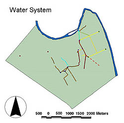 emains. In the southeast corner of
the ranch, behind the largest southern tank on the gravity system, there is a large
concrete water tank, which was once fed by a windmill.
None of the windmills are in use because the water they produce is too
salty for the cattle to drink. emains. In the southeast corner of
the ranch, behind the largest southern tank on the gravity system, there is a large
concrete water tank, which was once fed by a windmill.
None of the windmills are in use because the water they produce is too
salty for the cattle to drink.
Data, Maps and Graphics Produced
For the digitizing process, we were able to use the GPS data and the maps. Basic man-made water lines were digitized using the digital
orthophotos, wherever the acequia system was easy to identify. In the process, we created two
shapefiles to capture both point and line features. Both of these themes have attribute tables that show the characteristics of each component of the system.
[Back to Top] [Home]
[Topography]
[Geology and Geomorphology] [Soils]
[Land Cover and Vegetation]
[ Roads] [Water Resources]
[Cultural Features] [Land
Uses and Practices] [Home]
|
|
-- Original Data --
Original Data Sources - 1978
Maps and Aerial Photos
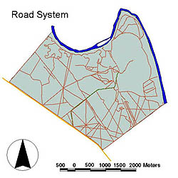
The
1978 maps showed various roads throughout the project site.
The roads were digitized using the rubbersheeted Geology map for the
northern portion of the site, and the rubbersheeted Vegetation map for the
southern portion of the site. (there
was no geology map for the southern portion)
The roads were categorized as follows for the ranch area:
The
more recent aerial photo (1998) showed many of the same roads, as well as many other roads
not shown on the 1978 maps.
Strategies for Field Verification
We used the GPS for field verification of the
roads shown on the aerial photo. Copies of the aerial photos
were produced and used as a map to find the roads
and make notes.
Strategies
for Additional Data Collection
We plan to map any additional roads we find by using
the GPS. Photos of the roads were
also taken using a camcorder so that we could refer later to the photos to
recall the conditions of various roads (degree of clearing, etc.)
-- Field Work --
The
person carrying the GPS device sat in the back of the pickup truck as we drove
on the roads around the project site. GPS data
was collected in the form of a line (string of data points) that will be overlaid in the GIS to
determine the map-accurate alignment of roads as seen on the aerial photos.
As we drove along the roads, we also took video using a camcorder with a
time stamp on it. The GPS also recorded the time as it collected coordinate
data. We noted the time difference
between the GPS and the camcorder so that we could later capture still images
from the camcorder tape at specific locations as recorded by the GPS.
In addition to the field
methods used, for future work we would recommend using the truck odometer as a backup method of
locating the placement of still images taken with the camcorder.
For instance, once we turned or went through a fence (known location on
the map), we could have reset the odometer in the truck and then every tenth of
a mile or so we could have recorded the distance by saying it into the
camcorder. This would have been a
useful backup method for locating where we took the video, because the GPS
device was only on part of the time we were taking video.
In addition, the line shape files created from the GPS only listed the
time at the beginning of each line recorded.
The GPS data will still be useable if we can show the roads as points,
where each X,Y,Z point has a time listed for when it was recorded.
-- Data and Maps Produced --
Field Data
The GPS data was the primary data taken on the field trips.
Most of the roads we traveled on were shown on the aerial photos.
In one area; however, there was a deer blind at the intersection of
several cleared senderos (paths, or deer shooting lanes) that were not shown on the aerial photos.
We drove to the deer blind, recording the road location using the GPS
instrument. There were several other roads leading up to the deer blind
that we did not record with the GPS, due to a lack of time and other priorities
for the trip. the roads we traveled on were shown on the aerial photos.
In one area; however, there was a deer blind at the intersection of
several cleared senderos (paths, or deer shooting lanes) that were not shown on the aerial photos.
We drove to the deer blind, recording the road location using the GPS
instrument. There were several other roads leading up to the deer blind
that we did not record with the GPS, due to a lack of time and other priorities
for the trip.
Comparison to Existing Data
Once the GPS data
were converted to the same coordinate system as the DOQQs, and the aerial photos
were rubbersheeted using the Image Analyst software, all of the data matched up almost
perfectly with the original data. There were several roads shown on the aerial photos that we
did not record using the GPS.
Data, Maps and Graphics Produced
Starting Point for Final Map Production
At first glance,
the line shapefiles produced with the GPS seemed to be a good starting
point for production of the final maps. This would reduce the error in the final map that might be
introduced by tracing lines from the GPS file, and it would reduce the amount of
work needed to produce the final map.
We decided to create a new file for the
roads, called "roads_2000" shapefile. However, because the
shapes created by the GPS conversion program were PolylineZ, they were not
easily convertible to other formats.
The first problem encountered was that ArcView's "Geoprocessing
Extension" will
not merge files with this type. In
an attempt to find another extension that would enable merging the files from the
two field trips, a search on the internet produced several editing programs,
e.g. Editing Tools Extension, that
looked promising. Unfortunately,
this program did not end up supporting PolylineZ shapes.
In addition, the ESRI viewer program ArcExplorer does not support
PolylineZ shapes at this time. This
may be an important program for future use of the data, because ArcExplorer is a
free viewer program that could potentially be used by the client or other
consultants for the project without requiring purchase of ArcView.
Based
on all of the limitations found with the PolylineZ shape type, it seemed most
logical to create a new shape file with regular Polylines.
This was done with the intention of providing future users of the
shapefile with a greater ability to use the data for various analyses (unknown
at this time), without being limited by the PolylineZ shape type.
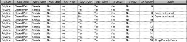
Road type classification
Within the
attribute table for the Polyline shape file created, the road type is listed
as both the Spanish Name and English Name. We
decided that the best breakdown for road
types would be the following:
-
Carretera
/ Highway (paved along the western
boundary)
-
Camino
/ Ranch Road (main dirt road to the ranch house)
-
Sereda
/ Cleared Path (dirt roads/cleared paths generally wide enough for one
vehicle)
The source of each road shown in the roads_2000 shape file (see screen capture
above) is listed in the attribute table. The
screen capture shown below is an example of what the attribute table looks like.
The data sources for each road are listed in the table.
GPS data from the 2nd trip was given
priority for digitizing because the GPS machine used on that trip was of very
high accuracy compared to the other data sources.
The DOQQ images matched up well with the GPS data, so the DOQQ image was
given the next highest priority for digitizing.
[Back to Top] [Home]
[Topography]
[Geology and Geomorphology] [Soils]
[Land Cover and Vegetation]
[ Roads] [Water Resources]
[Cultural Features] [Land
Uses and Practices] [Home]
|
|
-- Original Data -- 
Cultural features on the 1978 maps were difficult to note and
were considered unreliable because they were marked by small black
unlabeled dots on the paper. These were
assumed to be buildings or ranch facilities, but field observation was
required for verification. In addition to the black dots, the two towns
of Hidalgo and Colombia were observable on the outer edges of the study
area.
-- Field Work --
In the
field we identified the mapped dots largely as worker residences, open walled
agricultural storage buildings and work sheds.
We used the hand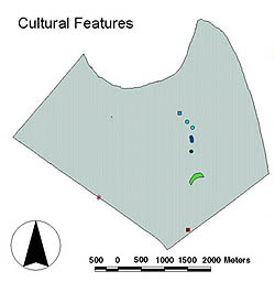 held GPS device to
locate the exact position of a new residence which was constructed since 1978. We also found the
ruins of a house in the southeast quadrant of the ranch, estimated to be
approximately 60 or 70 years old (not noted on the paper maps). This was also
located with the GPS unit. held GPS device to
locate the exact position of a new residence which was constructed since 1978. We also found the
ruins of a house in the southeast quadrant of the ranch, estimated to be
approximately 60 or 70 years old (not noted on the paper maps). This was also
located with the GPS unit.
-- Data and Maps Produced --
Although the cultural features data were not very extensive, field notes
and GPS files were used to create
a point theme marking the location of the above
mentioned structures.
[Back to Top] [Home]
[Topography]
[Geology and Geomorphology] [Soils]
[Land Cover and Vegetation]
[ Roads] [Water Resources]
[Cultural Features] [Land
Uses and Practices] [Home]
|
|
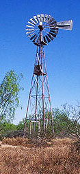 -- Original Data -- -- Original Data --
Though several land use features were described on
the 1978 vegetation maps (cultivated, induced and natural pasture, and
ranchland) there was no formal land use map for the area at the time.
-- Field Work --
During the field trips, meetings with the ranch
foreman and owner revealed a variety of agricultural uses on the land.
Our own observations confirmed and expanded what was evident on the 1978
vegetation map.
-- Data and Maps Produced -- 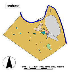
For the creation of the 2000 land use map, a different scheme
was chosen to describe the study area. We used the Anderson
land use, land cover classification system for remote sensor data,[1]
published on the USGS website. Not all of Anderson's classification
units
apply to the ranch, however, so the team created a modified version
(see below), carried out to the third level and adapted for the
specifics of this site. Using GPS data, field notes and aerial photographic interpretation,
all the land area within the ranch was classified and digitized for use as
a polygon theme.
Landuse
Classification System For Rancho San Eduardo
Based on Anderson's landuse /land cover classification system for
remote sensor data |
| Level
I |
Level
II |
Level
III |
| 1. Urban or built-up land |
11. Residential
14. Transportation,
communications, and utilities
17. Other urban or
built-up land |
|
| 2. Agricultural land |
21.
Cropland and pasture
22. Orchards,
groves, ornamental horticulture
23. Other
agricultural land |
|
| 3. Rangeland |
31.
Herbaceous rangeland
32. Shrub and brush rangeland
33. Mixed rangeland |
|
| 4. Water |
41. Streams and canals
42. Reservoirs
43. River |
411.
Arroyos
421. Livestock Tank |
| 5. Wetland |
52
Non forested wetland |
|
| 6. Barren land |
61.
Beaches
62. Bare exposed
rock
63. Mixed barren
land |
631. Badlands |
References
[1] http://ca.water.usgs.gov/pnsp/circ1131/table1.html
[Back to Top] [Home]
[Topography]
[Geology and Geomorphology] [Soils]
[Land Cover and Vegetation]
[ Roads] [Water Resources]
[Cultural Features] [Land
Uses and Practices] [Home]
Continue
to
Maps |
|