Modeling Methodology

Technical Model-Building Methodology
The following general methodology was used to create all three land suitability models using ArcView's ModelBuilder software.

Once the variables of each model were determined (as described above), the shapefiles with the source data were modified to reflect the attributes that would be given consideration (e.g. adding a buffer to a given attribute).
In ArcView, the ModelBuilder Extension was activated, and the modified shapefiles with appropriate legends were pulled into a new View.
The ModelBuilder feature was activated and the diagram of the model was developed.
All input shapefiles had to be converted to grid files. The latter are composed of pixels (square cells), to which one can assign different values. The model software processes such values to derive results.
Each input shapefile was converted to a discrete grid format using the Vector Conversion function. Using ModelBuilder, the cell size selected was 10 meters, the extent of theme was the property boundary, and the evaluation scale selected was 1-100.
In some cases it was necessary to create a grid themes from two or more discrete grid inputs. In order to do this, the Arithmetic Overlay function was used.

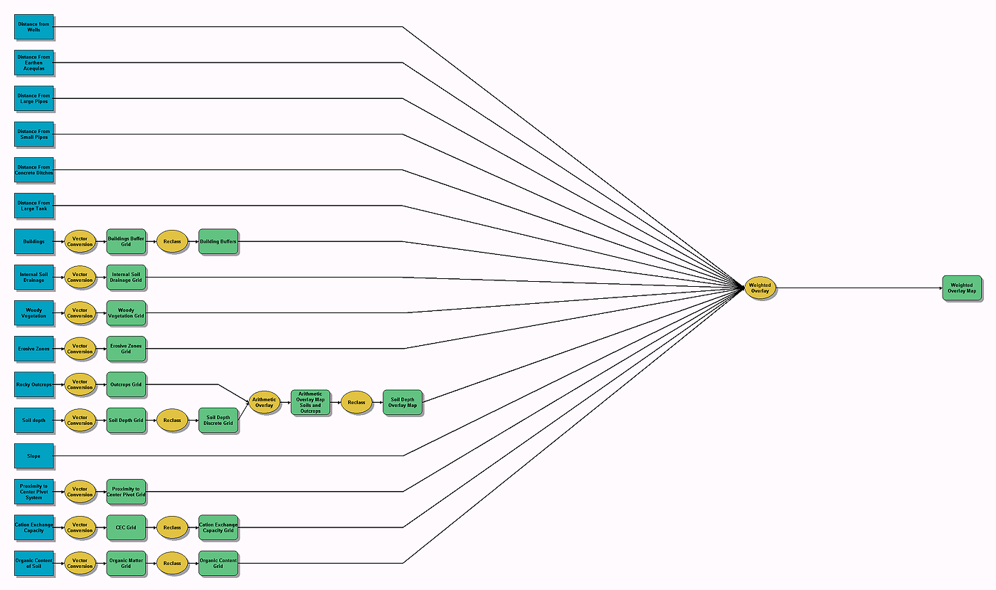
The "Arithmetic Overlay" allows the modeler to combine several input grid themes by assigning an operator and multiplier to each scheme. The main advantage is that it allows Boolean manipulation to scale and calculate intersections and overlapping areas.

Example: I have two input files "floodplain" and "riverbanks." We want to know which areas are

inside the floodplain but above the riverbanks, and
inside the floodplain and part of the riverbanks

To this end, the following values are assigned to specific areas:

For Floodplains	For Riverbanks
0 = not in floodplain 1 = in floodplain	1 = not in riverbanks 2 = in riverbanks

If we multiply the values of each grid cell, the result consist of 0s, 1s, and 2s which mean:

0 =	not in floodplain, regardless of whether outside or inside the riverbank
1 =	in floodplain and not in riverbanks
2 =	in floodplain and in riverbanks

Because the output grids of the Arithmetic Overlay are continuous, these had to be converted to discrete grid themes using the Reclassification function.

The Reclassification Process allows you to group cell values into classes. Classes are defined by specifying the values each class will contain. The input data for the reclassification is a grid theme. The output theme is a grid theme containing the newly defined classes.

Once all the grid themes were complete, they were connected to a Weighted Overlay.

The Weighted Overlay Process allows you to combine data from several input grid themes by converting their cell values to a common scale, assigning a weight (percent influence) to each theme, and giving a weighted value to each attribute considered.

Each category in the grid themes used in the models was assigned a numerical value, or "influence value," ranging from 0 to 100 according to criteria established by the team. By assigning a value to each category, one translates its degree of importance to a format that the computer software can use to run a model. Categories with high values are given a high degree of importance, while categories with low values are given low importance. These values were assigned to each theme category with the Weighted Overlay function of the ModelBuilder. In addition to establishing a value for each category, each variable (grid theme) considered in the model was assigned a percent value to reflect its degree of influence in the model. To run the model, all values must add up to 100. The variables that influence the model the most are given the highest percentage.

Once the connections to the Weighted Overlay were established, the models were run to produce shapefiles showing zones of varying suitability for human settlement, agriculture and preservation.

Notes:
The assignment of NODATA status to areas outside the study area was handled differently in the agriculture model. Remember, areas outside a feature to be valued were labeled with the NODATA option in the weighted overlay process. In the other models, we always produced shapefiles that had polygons covering the whole area, but this was not the case for agriculture. If, for example, there was a buffer around a well, the shapefile in the agriciulture model would contain only the buffer area; whereas for the settlement or preservation model, we had shapefiles containing the buffer area AND the area outside the buffer to the extent of the property area.

What does this difference mean? The results for both approaches are the same, as long as the model is only applied to the property area. As soon as the model would, for whatever reason, be extended, let's say to include adjacent properties, one would have to produce a shapefile similar to those used for the settlement or preservation models.

This modified process also seemed to reveal an error in the ModelBuilder program. When the model is saved under a different name, the program sets back all the "Restricted" values to zero. If the "NO DATA" area has been set to "Restricted" (meaning that the area is taken out of the weighing process completely and left blank) it must be re-set to this value after saving it under another name.

____
The main explanations in italics were taken as quotes from the respective ModelBuilder wizards.